Saddle Points and Stochastic Gradient Descent

Essentially all machine learning models are trained using gradient descent. However, neural networks introduce two new challenges for gradient descent to cope with: saddle points and massive training sets. In this post we describe how these two challenges conspire together to create deadly traps, and we discuss means to escape them.

Background: Optimizing a loss function:

Machine learning algorithms attempt to model observed data in order to predict properties about unobserved data, and in most cases they do this by:

1. Parametrizing a space of models (with some parameters \(\vec{\bf{x}} = (x_1,\dots, x_m)\)),
2. Defining a loss function \(f(\vec{\bf{x}})\to \mathbb{R}\) which measures the total error between the model at parameters \(\vec{\bf{x}} = (x_1,\dots, x_m)\) and the observed data,
3. Finding the optimal parameters \(\vec{\bf{x}} = (x_1,\dots, x_m)\) which minimize the loss.

Assuming we’ve completed steps (1) and (2), the question then becomes: How do we minimize a high dimensional function \(f(\vec{\bf{x}})\to \mathbb{R}\)?

We use gradient descent:

Although there are many possible ways to minimize a function, by and far the most successful approach for machine learning is to use gradient descent. This is a greedy algorithm, where we make an initial first guess \(\vec{\bf{x}}_0\) for the optimal parameters, and then iteratively modifying that guess by moving in the direction in which \(f\) decreases most quickly, that is:

\[\vec{\bf{x}}_n = \vec{\bf{x}}_{n-1} - \nabla f\]

(where \(\nabla f\) denotes the gradient of \(f\)). With some basic assumptions, the sequence of guesses \(\vec{\bf{x}}_0, \vec{\bf{x}}_1, \vec{\bf{x}}_2, \vec{\bf{x}}_3, \dots\) can be shown to improve steadily, and if \(f\) is sufficiently nice (for example if \(f\) is strongly convex), then this sequence will converge to a (local) minimum of \(f\) fairly quickly.

Saddle points

We now introduce the first villain in our saga, saddle points, which are known to cause problems for gradient descent. A saddle point is a critical point¹ of a function which is neither a local minima or maxima.

Locally, up to a rotation and translation, any function \(f\) is well approximated near a saddle point by

\[\overset{concave} {\overbrace{\frac{-a_1}{2}x_1^2+\dots +\frac{-a_k}{2}x_k^2}} + \overset{convex}{\overbrace{\frac{a_{k+1}}{2}x_{k+1}^2+\dots+\frac{a_m}{2}x_m^2}}\]

where \(1<k<m\) and all \(a_i>0\), and the translation sends the saddle point to the origin.

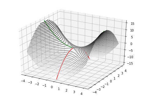
Gradient descent proceeds extremely slowly near a saddle point.

Why? Well, \(\nabla f=0\) at a saddle point \(\vec{\bf{x}}\) so the gradient \(\nabla f\simeq 0\) will be extremely small near the saddle point. Recall that each gradient descent update is given by \(\vec{\bf{x}}_n = \vec{\bf{x}}_{n-1}- \nabla f\). So \(\vec{\bf{x}}_n \simeq \vec{\bf{x}}_{n-1}\), and each update barely improves the current guess. You can see this quite clearly in the following picture:

Nevertheless, if we choose \(\vec{\bf{x}}_0\) randomly, then almost certainly:

Gradient descent will (eventually) escape saddle points

Recall the gradient descent formula \[\vec{\bf{x}}_n = \vec{\bf{x}}_{n-1} +\Delta \vec{\bf{x}}_{n-1}, \quad \text{ where } \quad \Delta \vec{\bf{x}}= - \nabla f\] in coordinates, this reads: \[\Delta x_i = - \frac{\partial f}{\partial x_i}\]

Meanwhile the local model for a saddle point at the origin is: \[f(x_1,\dots,x_n) = \overset{concave} {\overbrace{\frac{-a_1}{2}x_1^2+\dots +\frac{-a_k}{2}x_k^2}} + \overset{convex}{\overbrace{\frac{a_{k+1}}{2}x_{k+1}^2+\dots+\frac{a_m}{2}x_m^2}}\]

Now, we have \[\frac{\partial f}{\partial x_i} = -a_ix_i\quad \text{ for } i<=k\quad\quad \text{ and }\quad\quad\frac{\partial f}{\partial x_i} = a_ix_i\quad \text{ for } i>k\]

So: \[\Delta x_i = a_ix_i \quad \text{ for } i<=k \quad \text{ (repulsive dynamics)}\] and \[\Delta x_i = -a_ix_i \quad \text{ for } i>k \quad \text{ (attractive dynamics)}\]

Though we are attracted to the saddle point in some directions, we are eventually ejected from the saddle point by the repulsive forces. Indeed it can be shown that with random initialization, we will almost surely escape²

Finally, we should emphasize that there are lots of saddle points in deep neural networks.

Typically, the loss function in deep neural networks is noisy

For most machine learning algorithms, the loss function can be written as a sum over the training data:

\[ f(\vec{\bf{x}}) = \sum_j^N f_j(\vec{\bf{x}}),\]

where \(N\) is the number of training samples, and each \(f_i(\vec{\bf{x}})\) measures the model’s error on the \(i\)-th training sample. Now, deep neural networks need massive data sets to train successfully, and so it is extremely costly to evaluate the loss over the entire training set. Instead, one typically approximates the loss on a randomly chosen minibatch \(J\subset \{1,\dots, N\}\) of data, \[ f_{J-approx}(\vec{\bf{x}}) = \sum_{j\in J} f_j(\vec{\bf{x}}).\] This subsampling from the training data results in a noisy loss function.

In turn, we modify the gradient descent algorithm as follows: on iteration, we choose a random minibatch \(J\subset \{1,\dots, N\}\) and update our previous guess by: \[\vec{\bf{x}}_n = \vec{\bf{x}}_{n-1} +\Delta \vec{\bf{x}}_{n-1}, \quad \text{ where } \quad \Delta \vec{\bf{x}}= - \nabla f_{J-approx}\] It is worthwhile noting that minibatches chosen randomly at each iteration are mutually independent. The resulting algorithm is known as stochastic gradient descent.

Adding this noise, however, can have some surprising consequences near saddle points:

Example:

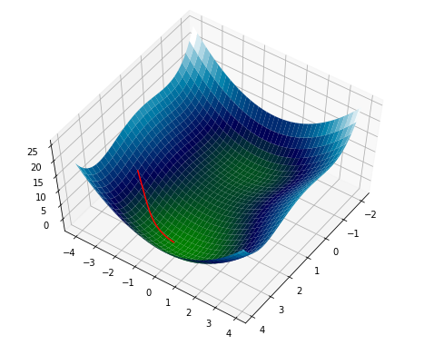
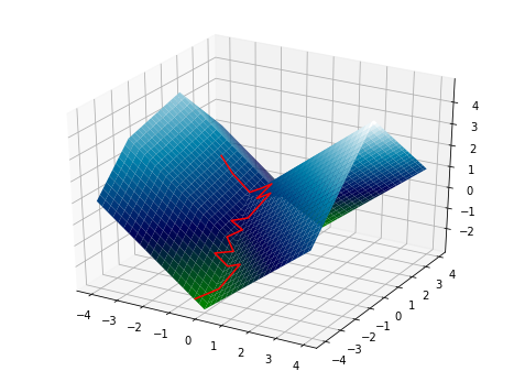
Consider the following function, standard gradient descent does an excellent job of finding the minimum:

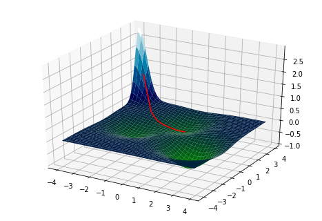
Now, we will add some noise³. Notice that it doesn’t roll immediately into the basin, but lingers along the ridge somewhat.

Adding more noise⁴ causes it to converge fairly rapidly to the saddle point between the two minima.

What is going on here? How can noise cause gradient descent to become trapped at saddle points?

Why noise hurts

To simplify our discussion, we will restrict ourselves to one of the concave down principal axes of the saddle point - along which the dynamics ought to be repulsive - in which case the local model becomes one dimensional: \[f(x)= -ax^2.\] with \(a\) positive. The corresponding local model for the noisy loss function is: \[f(x)=-(a+\xi)x^2 - \eta x\] where \(\xi\) and \(\eta\) are mean zero random variables encoding the noisy measurement of the coefficients of \(x^2\) and \(x\) in the Taylor expansion (note that \(f\) is now a random variable as well).

So, we have \[\frac{\partial f}{\partial x} = -ax -\xi x-\eta\] And the gradient descent update becomes: \[\Delta x =a x+ \xi x+\eta\]

Let’s consider the separate components \[ \Delta x = \overset{\text{Usual gradient}}{\overbrace{ax}} +\overset{\text{Attractive noise}}{\overbrace{\xi x}}+\overset{\text{Diffusive noise}}{\overbrace{\eta}}\]

Attractive noise:

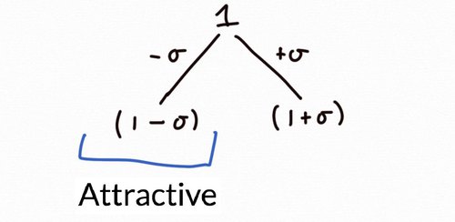
Let’s start by considering the attractive noise in isolation, ie. \(\Delta x = \xi x\). The corresponding update is \[x_{n+1}=x_n + \xi x_n = (1+\xi) x_{n}\]

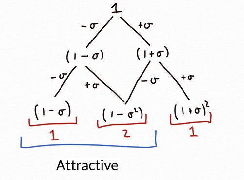
Suppose that we flip a coin at each iteration and \(\xi\) equals \(\sigma\) if we get heads or \(-\sigma\) if we roll tails. Then after 1 iteration, \(x\) is rescaled by either a factor of \(1-\sigma\) or \(1+\sigma\) (with equal probability). We picture the possible transitions below:

Next, consider what the possiblilities are after two iterations: \(x\) is rescaled by a factor of either

1. \((1-\sigma)^2\) if we roll two tails (with probably \(\frac{1}{4}=\frac{1}{2}\times \frac{1}{2}\))
2. \((1-\sigma^2)=(1-\sigma)(1+\sigma)\) in two distinct ways: we roll either a heads and then a tails or vice versa (with total probability \(\frac{1}{2} = 2\times(\frac{1}{2}\times \frac{1}{2})\))
3. \((1+\sigma)^2\) if we roll two tails (with probably \(\frac{1}{4}=\frac{1}{2}\times \frac{1}{2}\))

Since the first two scaling factors are both less than one, \(\lvert x_2\rvert<\lvert x_0\rvert\) with probability \(\frac{3}{4}\).

Continuing like this we see that \(\lvert x_4\rvert<\lvert x_0\rvert\) with probability at least \(\frac{11}{16}\).

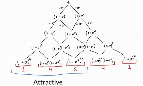
Indeed we see that the mode of \(x_n\) - for which we expect an equal number of heads and tails, namely \(n/2\) - is \[(1-\sigma)^{n/2}(1+\sigma)^{n/2}x_0=(1-\sigma^2)^{n/2}x_0,\] and \(x_n\) gravitates towards zero⁵ at an average rate of \[\frac{1}{n}(-\sigma^2\frac{n}{2})=-\frac{\sigma^2}{2}.\]

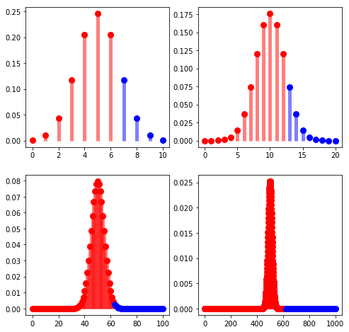
In fact, we have \(\lim_{n\to\infty} x_n = 0\) with probability 1. The figure below illustrates this trend for larger and larger \(n\).

Diffusive noise:

Recall: \[ \Delta x = \overset{\text{Usual gradient}}{\overbrace{ax}} +\overset{\text{Attractive noise}}{\overbrace{\xi x}}+ \overset{\text{Diffusive noise}}{\overbrace{\eta}}\]

So the diffusive component is: \[ \Delta x = \eta\]

If we isolate the diffusive compenent, then after \(N\) iterations we have \[x_N=x_0+\sum_{n=0}^N \Delta x_n = x_0+\sum_{i=0}^N \eta_i\]

Here \(\eta_i\) are iid random variables with mean zero. If we assume the standard deviation of \(\eta_i\) is \(\tau\) then by the central limit theorem, \(\sum_{i=0}^N \eta_i\sim N(0, \tau\sqrt{N})\). Therefore:

\[x_N\sim N(x_0, \tau\sqrt{N})\]

In summary, \(x\) diffuses at a rate of \(\tau\sqrt{N}\).

Does the diffusive or attractive noise dominate?

Consider again the model for stochastic gradient descent localized around a saddle point:

\[ \Delta x = \overset{\text{Usual gradient}}{\overbrace{ax}} +\overset{\text{Attractive noise}}{\overbrace{\xi x}} +\overset{\text{Diffusive noise}}{\overbrace{\eta}}\]

Since the intensity of the attractive noise is proportional to \(x\), it’s clear that the attractive noise dominates the behavior for sufficiently large values of \(x\), while the diffusive noise dominates the behavior for sufficiently small values of \(x\).

This describes the behavior at the two extremes. However, further direct analysis of the behavior is hampered by our not knowing anything about the random variables \(\xi\) or \(\eta\). Fortunately, if we assume they have finite moments, rescaled sums of independent draws of \(\xi\) and \(\eta\) limit to Brownian motion, and it makes sense to replace the finite difference equation above with the corresponding stochastic differential equation

\[dx = ax \:dt+\xi x \:dt +\eta\: dt\] where \(\xi\) and \(\eta\) are white noise whose correlation is time-independent.

Let \(\sigma\) and \(\tau\) represent the scaling factors such that \(W_t=\int_0^t\frac{\xi}{\sigma}\:dt\) and \(V_t=\int_0^t\frac{\eta}{\tau}\:dt\) are standard Brownian motion, and let \(\rho\) denote their correlation.⁶ Then we may write the equation as

\[dx = ax \:dt+\sigma x \:dW +\tau\: dU\]

Substituting \[\begin{align} \mu &= \frac{\tau\rho}{\sigma}, & \omega &= \tau\sqrt{1-\rho^2}, \text{ and }\\ V &= \frac{U-\rho W}{\sqrt{1-\rho^2}} & y&=x+\mu \end{align}\] yields the stochastic differential equation \[dy = a(y-\mu)\:dt +\sigma y\:dW+\omega\: dV\] where \(V\) and \(W\) are independent standard Brownian motions.

This equation has the following analytical solution:

\[y_t = y_0e^{(a-\frac{\sigma^2}{2})t+\sigma W_t}+\int_0^t e^{ (a-\frac{\sigma^2}{2})(t-s)+\sigma (W_t-W_s)}d\nu\] where \(\nu = \omega V_s-a\mu s\), as can be verified directly by differentiation (using Ito’s lemma).

In particular, we see that the attractive noise shifts the rate of exponential growth from \(a\) to \(a-\frac{\sigma^2}{2}\) .⁷ Thus, if \(a< \frac{\sigma^2}{2}\), then the growth rate becomes negative, namely the saddle point becomes attractive. Indeed, if there is no diffusive noise (i.e. \(\tau=0\)), the solution reduces to \(x_t = x_0e^{(a-\frac{\sigma^2}{2})t+\sigma W_t}\), which almost surely converges to zero.

Stationary distribution:

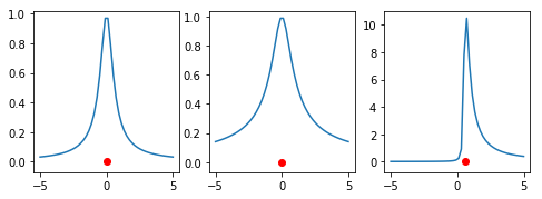
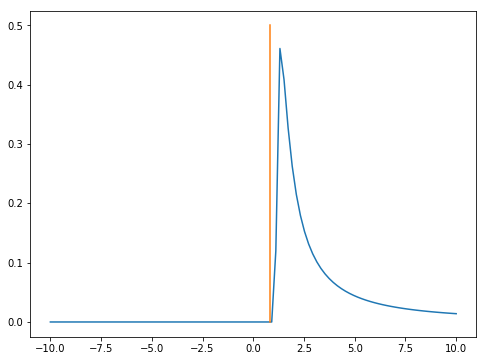
We would like to undestand the long term behaviour of \(x_t\). If \(a< \frac{\sigma^2}{2}\), then \(x_\infty:=\lim_{t\to\infty}x_t\) converges to a stationary distribution⁸. We solve for the stationary distribution in the appendix and find that the random variable \(x_\infty:=\lim_{t\to\infty}x_t\) is Pearson distributed. In particular, when \(\omega \neq 0\), \(x_\infty\) is governed by the following probability density:

\[p(y_\infty)=\frac{1}{Z}\left(\sigma^{2}y_\infty^{2} + \omega^{2}\right) ^{\frac{a}{\sigma^{2}} - 1} e^{- \frac{2 a \mu \operatorname{atan}{\left (\frac{ \sigma\, y_\infty}{\omega} \right )}} {\omega \sigma}}, \text{ where } x_\infty = y_\infty-\mu.\] Here \(Z\) is a normalizing constant (we will discuss the case where \(\omega=0\) in the next subsection).

Note that the random variable \(x_\infty\) is non integrable, which is to say its expected value is infinite. However, we do not expect \(x_t\) to diverge: for instance, for large \(R\), the odds that \(\lvert \lim_{t\to\infty}x_t \rvert > R\) become negligibly small: \[\mathbb{P}(\lvert \lim_{t\to\infty}x_t \rvert > R) = O\big(\big(\frac{1}{R}\big)^{1-\frac{2a}{\sigma^{2}}}\big)\text{ as } R\to \infty\]

Indeed, the mode of this distribution is at \(y = a\mu/(a-\sigma^2)\), which translates to \(x=\frac{\rho \sigma \tau}{a - \sigma^{2}}\).

Special Case 1: \(\xi\) and \(\eta\) are perfectly correlated

The special case where \(\omega=0\) corresponds to \(\xi\) and \(\eta\) being perfectly correlated. In this case \(y_\infty\) is Inverse Gamma-distributed⁹. To describe the distribution of \(x_\infty\), we may assume without loss of generality that \(\rho=1\). Then \(x_\infty+\tau/\sigma\) is an Inverse Gamma-distributed random variable with scale \(\beta = -2\frac{ a\tau}{\sigma^3}\) and shape \(\alpha = 1-2a/\sigma^2\).

Special Case 2: \(\xi\) and \(\eta\) are not correlated

In this case, \(\rho=0\), and \(x_\infty\) is Student’s t-distributed with \(\nu =1-\frac{2a}{\sigma^2}\) degrees of freedom, location \(\mu=0\), and scale \(\sqrt{\frac{\tau^2}{\sigma^2-2a}}\).

How should we escape saddle points in the presence of noise?

We can categorize some major strategies as follows:

• Decrease the attractive noise

  • Increase the minibatch size
  • Decrease/Anneal the learning rate
  • Stochastic Variance Reduction Gradient Descent

• Increase the diffusive noise

  • Perturbed Stochastic Gradient Descent

• Do not use a smooth loss function

  • Use ReLu’s

Basic means to escape saddle points:

Some basic methods to decrease the attractive noise are to:

• Increase the minibatch size.

  • Increasing the minibatch size by a factor of \(\alpha\) decreases the attractive noise by a factor of \(\frac{1}{\sqrt{\alpha}}\) which in turn decreases the odds of becoming stuck at the saddle point. In more detail, recall that the saddle point ceases to be attractive when \(\frac{\sigma^2}{2} < a\). Increasing the minibatch by a factor of \(\alpha\) scales \(\sigma\) to \(\frac{\sigma}{\sqrt{\alpha}}\). Thus for \(\frac{\sigma^2}{2a} < \alpha\), we expect to escape the saddle point. Unfortunately, the computational cost of each gradient step roughly increases by a factor of \(\alpha\) as well.

• Decrease/Anneal the learning rate.

  • Scaling the gradient descent updates by a learning rate of \(\frac{1}{\alpha}\) scales both \(a\) and \(\sigma\) by \(\frac{1}{\alpha}\). In particular, the saddle point will cease to be attractive if \(\frac{a}{\alpha}> \frac{1}{2}\big(\frac{\sigma}{\alpha}\big)^2\). Thus, for learning rates \(\frac{1}{\alpha}< \frac{2a}{\sigma^2}\), stochastic gradient descent should escape the saddle point. Indeed we will almost surely escape saddle points and succeed in converging to a local minima if we appropriately anneal the learning rate¹⁰. The downside is that if the learning rate is too small, training may take overly long (it roughly scales the training time by a factor of \(\alpha\)).

Stochastic Variance Reduction Gradient Descent

Stochastic Variance Reduction Gradient Descent (SVRG)¹¹ reduce the variance of stochastic gradient descent by modifying the procedure as follows: given a “landmark point” \(\tilde x\) and the full gradient \(\mathbb{E}(\nabla f(\tilde x))\) at that landmark, we make gradient updates at the location \(x\) using the following variance-reduced gradient: \[\nabla_{VR,\tilde x}\: f(x):= \nabla f(x) + \overset{SVRG-modification}{\overbrace{ \big(\mathbb{E}(\nabla f(\tilde x))-\nabla f(\tilde x)\big)}}.\] Notice that this modified “variance-reduced” gradient has the same expected value as the original noisy gradient, since the modification (the second term) has an expected value of zero. However, the variance of \(\nabla_{VR, \tilde x}\: f(x)\) is much less than \(\nabla f(x)\) when \(x\) is near \(\tilde x\), as becomes clear by regrouping the terms as follows: \[\nabla_{VR,\tilde x}\: f(x):= \overset{A}{\overbrace{ \big(\nabla f(x)-\nabla f(\tilde x)\big)}} + \overset{B}{\overbrace{\mathbb{E}(\nabla f(\tilde x))}}.\] Term \(B\) has zero variance, while term \(A\) is the difference of two postively correlated random variables, so it has low variance. Indeed, when \(x = \tilde x\), the variance of \(A\) is zero.

Since we need the landmark point \(\tilde x\) to be near \(x\), we simply update it periodically (for example at the start of every epoch).

Given that SVRG reduces the variance of the gradient, we should expect it to escape saddle points. Let’s analyze it from the perspective of the machinery developed above. We have: \[\begin{align} \nabla f(x) &= -ax \:dt-\sigma x \:dW -\tau\: dU,\\ -\nabla f(\tilde x) &= a\tilde x \:dt+\sigma \tilde x \:dW +\tau\: dU,\text{ and}\\ \mathbb{E}\big(\nabla f(\tilde x)\big) &= -a\tilde x \:dt\quad\text{ since }\mathbb{E}(dW)=\mathbb{E}(dU)=0\\ \end{align}\] so \[\nabla_{VR,\tilde x}\: f(x) = -ax \:dt-\sigma x \:dW + \sigma \tilde x \:dW,\] and the stochastic differential equation \(dx=-\nabla_{VR,\tilde x}\: f(x)\) becomes \[dx = ax \:dt+\sigma x \:dW +\tau' \:dW,\] where \(\tau'=- \sigma \tilde x\). We recognize this SDE as the special case where the attractive and diffusive noise are perfectly correlated; so \(x_\infty+\tau'/\sigma=x_\infty-\tilde x\) is an Inverse Gamma-distributed random variable with scale \(\beta = -2\frac{ a\tau'}{\sigma^3} = 2\frac{ a\tilde x}{\sigma^2}\) and shape \(\alpha = 1-2a/\sigma^2\). In particular, with probability 1, \[\lvert x_\infty\rvert >\lvert \tilde x\rvert,\] so we expect to move further from the saddle point every time we update the landmark point \(\tilde x\). Moreover, since the scale \(\beta\) of the inverse gamma-distribution is proportional to \(\tilde x\), heuristically, we expect the to escape no slower than gometrically in the updates of the landmark point, at a rate proportional to \(\beta/\tilde x = 2\frac{a}{\sigma^2}\).

Perturbed Stochastic Gradient Descent

Perturbed stochastic gradient descent¹² effectively increases the intensity \(\tau\) of the diffusive noise in the equation \[dx = ax \:dt+\sigma x \:dW +\tau\: dU\] while keeping the intensity \(\sigma\) of the attractive noise as well as the deterministic growth rate \(a\) fixed. In particular, \(x_\infty\) remains Pearson distributed.

Since the scale of the distribution of \(x_\infty\) depends linearly on \(\tau\), it follows that \(x_\infty\) will disperse proportionately. Thus, if we rescale \(\tau\) by a factor of \(\alpha\), then, intuitively, \(\mathbb{P}(\lvert \lim_{t\to\infty}x_t \rvert < R)\) will scale on the order of \(\frac{1}{\alpha}\).

In a practical setting, the loss function will only be well approximated by the local saddle point model within a finite radius \(R\) of the saddle point, so the odds of being trapped there will decrease roughly by a factor of \(\frac{1}{\alpha}\). Summarizing this heuristic analysis, Perturbed Stochastic Gradient Descent should be an effective means of escaping saddle points in the setting of a noisy loss function.

Use ReLu’s

Regularized linear units result in piecewise linear loss functions. In theory, this dramatically changes the dynamics and eliminates the attractive noise in the local update equation (though some diffusive noise may remain). In practice, if the piecewise linear loss function is sufficiently fine and well approximated by a smooth loss, then the above analysis may still indicate that the noise may cause stochastic gradient descent to suffer near saddle points. Of course, it would be worthwhile to investigate the situation further.

Open questions

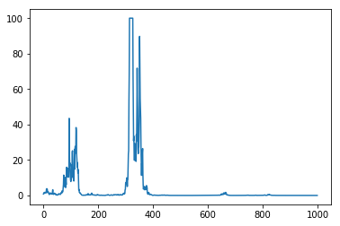
In this post we examined the impact of noise on stochastic gradient descent near saddle points by looking at the limiting \(t\to\infty\) stationary distribution. However, the local model \[f(\vec{\bf{x}}) \simeq \frac{\pm a_1}{2}x_1^2+\dots +\frac{\pm a_m}{2}x_m^2\] for the loss function near a saddle point is just that: a local model. In practice, there will be a radius \(R\) outside of which the local model is no longer an accurate approximation of loss function. It would be worthwhile exploring when trajectories \(x_t\) of the stochastic differential equation \[dx = ax \:dt+\sigma x \:dW +\tau\: dU\] first exceed \(R\) in absolute value. For instance, the following plot gives an example of such a trajectory; notice that while it spends much of its time near zero, it makes some occasional very large forays away from zero; any such foray might be sufficient to escape the saddle point.

In future work we would also like to explore whether or not saddle points in typical neural networks have strong attractive noise, and how the size and depth of such networks affects the intensity of that attractive noise. For instance, there need only be a single strongly repulsive direction from a saddle point in order to escape; perhaps increasing the dimensionality of a network also increases the odds that such a direction exist.

I work at the Human Diagnosis Project. We are looking for researchers and engineers who think outside the box.

Appendix A: Solving for the stationary distribution

The Fokker-Planck equation equation says that the probability density \(p(y, t)\) to the stochastic differential equation \[dy = a(y-\mu)\:dt +\sigma y\:dW+\omega\: dV\] solves the PDE \[{\frac {\partial }{\partial t}}p(y, t)=-{\frac {\partial }{\partial y}}\left[A (y)p(y,t)\right]+{\frac {\partial ^{2}}{\partial y^{2}}}\left[D(y)p(y,t)\right],\] where \(A(y) = a(y-\mu)\) and \(D(y)=\frac{1}{2}(\sigma^2 y^2+\omega^2)\). For a stationary distribution, the time derivative on the left-hand-side vanishes. Thus, we have \(\frac {\partial }{\partial y}J(y) = 0\), where \[J(y)=-A(y)p(y) +\frac{\partial}{\partial y} [D(y)p(y)].\] Since \(J\) is constant and both \(p\) and \(\frac {\partial p}{\partial t}\) vanish at \(\infty\), we must have \(J(y)=0\), which yields the ODE: \[\frac{\partial}{\partial y} [D(y)p(y)]=A(y)p(y).\] This, in turn, can be solved by standard techniques to find the solution \[\left(y^{2} \sigma^{2} + \omega^{2}\right) ^{\frac{a}{\sigma^{2}} - 1} e^{- \frac{2 a \mu \operatorname{atan}{\left (\frac{y \sigma}{\omega} \right )}} {\omega \sigma}},\] up to a constant multiple. From the ODE, we also see that \[A(y)-\frac{\partial D(y)}{\partial y} =0 \quad\quad\Leftrightarrow\quad\quad \frac{\partial p(y)}{\partial y}=0,\] which leads to the linear equation \(0= y(a- \sigma^{2}) - a\mu\) for the mode of \(p\).

---

1. That is \(\vec{\bf{x}}\) is a critical point if \(\nabla f=0\) at \(\vec{\bf{x}}\). Said differently \(f\) is flat to first order near \(\vec{\bf{x}}\).↩

2. Lee JD, Simchowitz M, Jordan MI, Recht B. Gradient Descent Converges to Minimizers. 2016;(Equation 1):1–11.↩

3. By gently shaking the surface: that is, we translate it by a normally distributed random variable with standard deviation 1.↩

4. By shaking the surface: that is, we translate it by a normally distributed random variable with standard deviation 2.↩

5. On the other hand, the average value of the scaling factors is 1. Indeed the expected value of \(x_n\) is \(x_0\) for all \(n\).↩

6. So for any times \(t\) and \(s\), the variances are \(\mathbb{E} \big((W_t-W_s)^2\big)=(t-s)\), and \(\mathbb{E}\big((U_t-U_s)^2\big)=(t-s)\), while the correlation is \(\mathbb{E}\big((W_t-W_s)(U_t-U_s)\big) = \rho(t-s)\).↩

7. Note that \(-\frac{\sigma^2}{2}\) is the same convergence rate that appeared in the discrete case.↩

8. Dufresne D. The distribution of a perpetuity, with applications to risk theory and pension funding. Vol. 1990, Scandinavian Actuarial Journal. 1990. p. 39–79.↩

9. Dufresne D. The distribution of a perpetuity, with applications to risk theory and pension funding. Vol. 1990, Scandinavian Actuarial Journal. 1990. p. 39–79.↩

10. Pemantle R. Nonconvergence to unstable points in urn models and stochastic approximations. Ann Probab [Internet]. 1990;18(2):698–712. Available here.↩

11. Johnson R, Zhang T. Accelerating Stochastic Gradient Descent using Predictive Variance Reduction. Proc Conf Neural Inf Process Syst [Internet]. 2013;1(3):315–23. Available here↩

12. Jin C, Ge R, Netrapalli P, Kakade SM, Jordan MI. How to Escape Saddle Points Efficiently. 2017;1–35. Available here↩

Site proudly generated by Hakyll