Bayesian Optimization Exploration
A short exploration of using bayesian optimization to make a good choice of hyperparameters. The detailed jupyter notebook can be found in RegressionWithBayesOpt.ipynb.
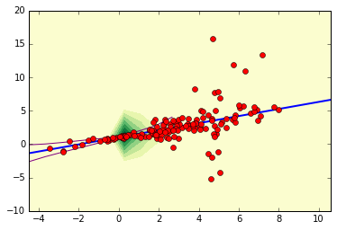
Consider the following data set (pictured at two separate scales):
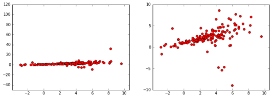
There seems to be a linear relationship between \(x\) and \(y\), and the \(y\)-values seem to concentrate near \(x=0\) and disperse for large values of \(x\). We want to model the data near \(x=0\) via the following model
\[y=ax+b+\epsilon\]
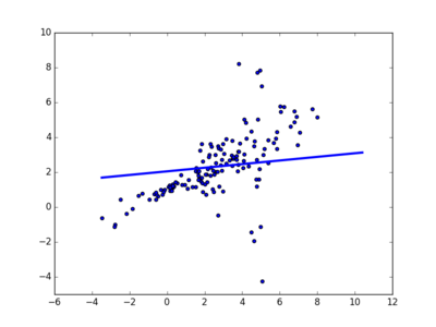
where \(\epsilon\) is noise which depends on \(x\). Notice that there are some extreme outliers, so using a least-squares approach doesn’t lead to a good fit:
We need \(\epsilon\) to heavy-tailed; so we fit a student t distribution (where the mode, scale, and shape all depend on \(x\)) using gradient descent.
Of course, this is a toy problem, which we are playing with because it is simple to visualize; this exploration is really about Bayesian optimization: The challenge is that we won’t acheive a good fit without proper regularization, and we then need to choose hyperparameters \(\lambda_1,\dots,\lambda_n\) to control the regularization. For any given choice of hyperparameters, we can fit our model on a training subset of the data, and then evaluate the fit on a cross-validation subset of data leading to an error function:
\[\varepsilon_{CV}(\lambda_1,\dots,\lambda_n):=\textrm{CrossValidationError}(\lambda_1,\dots,\lambda_n)\]
which we want to minimize. To minimize this we could use:
- A grid search for optimal values of \(\lambda_1,\dots,\lambda_n\),
- A random search for optimal values of \(\lambda_1,\dots,\lambda_n\),
- Numerical Optimization (such as Nelder-Mead),
- Bayesian Optimization.
Note that sampling \(\varepsilon_{CV}\) at a choice of hyperparameters can be costly (since we need to fit our model each time we sample); so rather than sampling \(\varepsilon_{CV}\) either randomly or on a grid, we’d like to make informed decisions about the best places at whcih to sample \(\varepsilon_{CV}\). Numerical Optimization and Bayesian Optimization both attempt to make these informed decisions, and we focus on Bayesian Optimization in this tutorial.
The basic idea is as follows: we will sample \(\varepsilon_{CV}\) at a relatively small number of points, and then fit a gaussian process to that sample: i.e. we model the function \(\varepsilon_{CV}(\lambda_1,\dots,\lambda_n)\) (pictured in red):
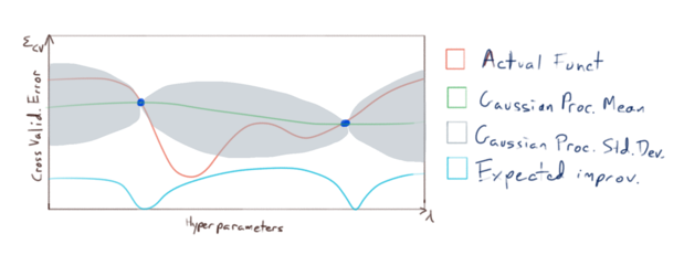
This model give us estimates of both
- the expected (mean) value of \(\varepsilon_{CV}\) if we were to sample it at novel points (pictured in green), as well as
- our uncertainty (or expected deviation) from that mean (the region pictured in grey),
and we use this information to choose where to sample \(\varepsilon_{CV}\) next. Now it is important to note that our primary concern is not to accurately model \(\varepsilon_{CV}\) everywhere with our gaussian process; our primary concern is to accurately model \(\varepsilon_{CV}\) near it’s minimums. So we sample \(\varepsilon_{CV}\) at points where we have the greatest expected improvement of fitting our model to the minimums of \(\varepsilon_{CV}\):
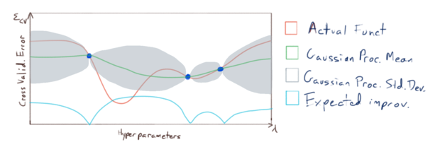
and we repeat until our model fits \(\varepsilon_{CV}\) accurately enough near it’s minimums:
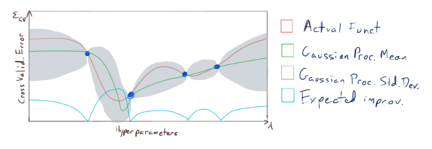
Finally, we use the resulting model to make an optimal choice for our hyperparameters \(\lambda_1,\dots,\lambda_n\).
This leads to a much better fit (green is the probability density, purple is one standard deviation - only when defined):
The full tutorial (with lots of comments and details) can be found in the jupyter notebook RegressionWithBayesOpt.ipynb.